Rabinovich-Fabrikant equations
The Rabinovich–Fabrikant equations are a set of three coupled ordinary differential equations exhibiting chaotic behaviour for certain values of the parameters. They are named after Mikhail Rabinovich and Anatoly Fabrikant, who described them in 1979.
\[\begin{split}\begin{aligned}
&\dot{x}=y\left(z-1+x^{2}\right)+\gamma x \\
&\dot{y}=x\left(3 z+1-x^{2}\right)+\gamma y \\
&\dot{z}=-2 z(\alpha+x y)
\end{aligned}\end{split}\]
where \(\alpha, \gamma\) are constants that control the evolution of the system.
https://zh.wikipedia.org/wiki/拉比诺维奇-法布里康特方程
https://en.wikipedia.org/wiki/Rabinovich%E2%80%93Fabrikant_equations
[1]:
import brainpy as bp
import matplotlib.pyplot as plt
[2]:
@bp.odeint(method='rk4')
def rf_eqs(x, y, z, t, alpha=1.1, gamma=0.803):
    dx = y *(z-1+x*x) + gamma *x
    dy = x *(3*z+1-x*x) + gamma *y
    dz = -2*z*(alpha+x*y)
    return dx, dy, dz
[3]:
def run_and_visualize(runner, duration=100, dim=3, args=None):
  assert dim in [3, 2]
  if args is None:
    runner.run(duration)
  else:
    runner.run(duration, args=args)

  if dim == 3:
    fig = plt.figure()
    ax = fig.add_subplot(111, projection='3d')
    for i in range(runner.mon.x.shape[1]):
      plt.plot(runner.mon.x[100:, i], runner.mon.y[100:, i], runner.mon.z[100:, i])
    ax.set_xlabel('x')
    ax.set_ylabel('y')
    ax.set_zlabel('z')
  else:
    for i in range(runner.mon.x.shape[1]):
      plt.plot(runner.mon.x[100:, i], runner.mon.y[100:, i])
    plt.xlabel('x')
    plt.xlabel('y')
  plt.show()
[4]:
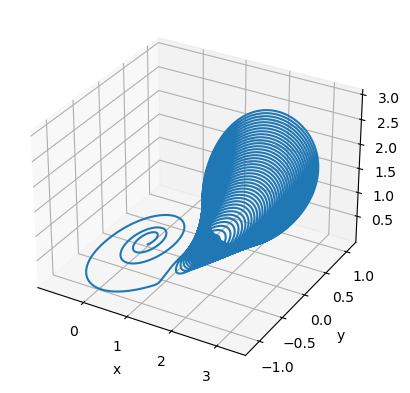
runner = bp.IntegratorRunner(
    rf_eqs,
    monitors=['x', 'y', 'z'],
    inits=dict(x=-1, y=0, z=0.5),
    dt=0.001
)
run_and_visualize(runner, 100, args=dict(alpha=1.1, gamma=0.87),)
WARNING:jax._src.lib.xla_bridge:No GPU/TPU found, falling back to CPU. (Set TF_CPP_MIN_LOG_LEVEL=0 and rerun for more info.)
[5]:
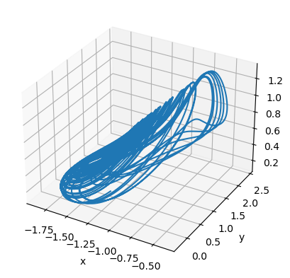
runner = bp.IntegratorRunner(
    rf_eqs,
    monitors=['x', 'y', 'z'],
    inits=dict(x=-1, y=0, z=0.5),
    dt=0.001
)
run_and_visualize(runner, 100, args=dict(alpha=0.98, gamma=0.1),)
[6]:
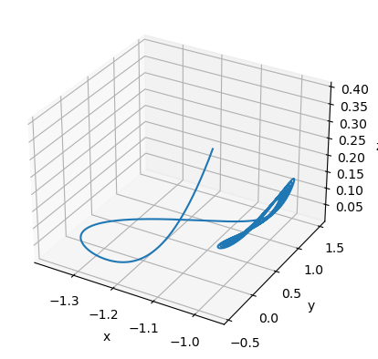
runner = bp.IntegratorRunner(
    rf_eqs,
    monitors=['x', 'y', 'z'],
    inits=dict(x=-1, y=0, z=0.5),
    dt=0.001
)
run_and_visualize(runner, 300, args=dict(alpha=0.14, gamma=0.1),)
[7]:
runner = bp.IntegratorRunner(
    rf_eqs,
    monitors=['x', 'y', 'z'],
    inits=dict(x=-1, y=0, z=0.5),
    dt=0.001
)
run_and_visualize(runner, 50, dim=2, args=dict(alpha=0.05, gamma=0.1),)
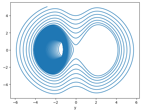
[8]:
runner = bp.IntegratorRunner(
rf_eqs,
monitors=['x', 'y', 'z'],
inits=dict(x=-1, y=0, z=0.5),
dt=0.001
)
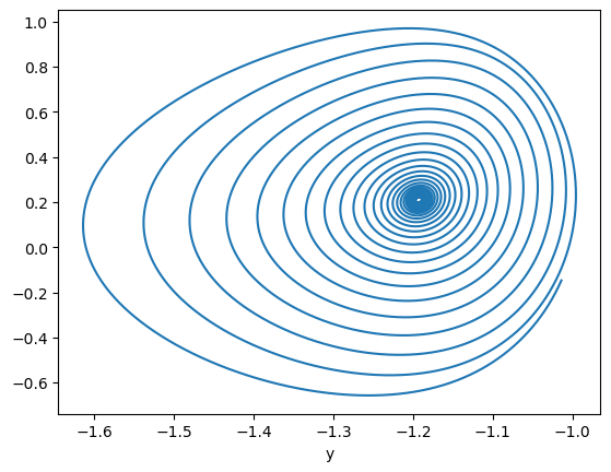
run_and_visualize(runner, 100, dim=2, args=dict(alpha=0.25, gamma=0.1),)
[9]:
runner = bp.IntegratorRunner(
rf_eqs,
monitors=['x', 'y', 'z'],
inits=dict(x=-1, y=0, z=0.5),
dt=0.001
)
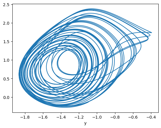
run_and_visualize(runner, 100, dim=2, args=dict(alpha=1.1, gamma=0.86666666666666666667),)
runner = bp.IntegratorRunner(
rf_eqs,
monitors=['x', 'y', 'z'],
inits=dict(x=-1, y=0, z=0.5),
dt=0.001
)
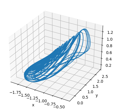
run_and_visualize(runner, 100, dim=3, args=dict(alpha=1.1, gamma=0.86666666666666666667),)
[10]:
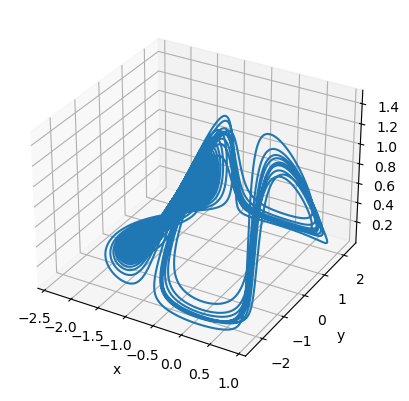
runner = bp.IntegratorRunner(
    rf_eqs,
    monitors=['x', 'y', 'z'],
    inits=dict(x=0.1, y=-0.1, z=0.1),
    dt=0.001
)
run_and_visualize(runner, 60, dim=3, args=dict(alpha=0.05, gamma=0.1),)