(Yang, 2020): Dynamical system analysis for RNN

Implementation of the paper:

• Yang G R, Wang X J. Artificial neural networks for neuroscientists: A primer[J]. Neuron, 2020, 107(6): 1048-1070.

The original implementation is based on PyTorch: https://github.com/gyyang/nn-brain/blob/master/RNN%2BDynamicalSystemAnalysis.ipynb

import brainpy as bp
import brainpy.math as bm
bp.math.set_platform('cpu')

import numpy as np
import matplotlib.pyplot as plt
from sklearn.decomposition import PCA

In this tutorial, we will use supervised learning to train a recurrent neural network on a simple perceptual decision making task, and analyze the trained network using dynamical system analysis.

Defining a cognitive task

# We will import the task from the neurogym library.
# Please install neurogym:
#
# https://github.com/neurogym/neurogym

import neurogym as ngym

# Environment
task = 'PerceptualDecisionMaking-v0'
kwargs = {'dt': 100}
seq_len = 100

# Make supervised dataset
dataset = ngym.Dataset(task, env_kwargs=kwargs, batch_size=16,
                       seq_len=seq_len)

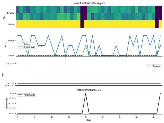
# A sample environment from dataset
env = dataset.env
# Visualize the environment with 2 sample trials
_ = ngym.utils.plot_env(env, num_trials=2, fig_kwargs={'figsize': (8, 6)})

input_size = env.observation_space.shape[0]
output_size = env.action_space.n
batch_size = dataset.batch_size

Define a vanilla continuous-time recurrent network

Here we will define a continuous-time neural network but discretize it in time using the Euler method.

\begin{align} \tau \frac{d\mathbf{r}}{dt} = -\mathbf{r}(t) + f(W_r \mathbf{r}(t) + W_x \mathbf{x}(t) + \mathbf{b}_r). \end{align}

This continuous-time system can then be discretized using the Euler method with a time step of \(\Delta t\),

\begin{align} \mathbf{r}(t+\Delta t) = \mathbf{r}(t) + \Delta \mathbf{r} = \mathbf{r}(t) + \frac{\Delta t}{\tau}[-\mathbf{r}(t) + f(W_r \mathbf{r}(t) + W_x \mathbf{x}(t) + \mathbf{b}_r)]. \end{align}

class RNN(bp.DynamicalSystem):
  def __init__(self,
               num_input,
               num_hidden,
               num_output,
               num_batch,
               dt=None, seed=None,
               w_ir=bp.init.KaimingNormal(scale=1.),
               w_rr=bp.init.KaimingNormal(scale=1.),
               w_ro=bp.init.KaimingNormal(scale=1.)):
    super(RNN, self).__init__()

    # parameters
    self.tau = 100
    self.num_batch = num_batch
    self.num_input = num_input
    self.num_hidden = num_hidden
    self.num_output = num_output
    if dt is None:
      self.alpha = 1
    else:
      self.alpha = dt / self.tau
    self.rng = bm.random.RandomState(seed=seed)

    # input weight
    self.w_ir = bm.TrainVar(bp.init.parameter(w_ir, (num_input, num_hidden)))

    # recurrent weight
    bound = 1 / num_hidden ** 0.5
    self.w_rr = bm.TrainVar(bp.init.parameter(w_rr, (num_hidden, num_hidden)))
    self.b_rr = bm.TrainVar(self.rng.uniform(-bound, bound, num_hidden))

    # readout weight
    self.w_ro = bm.TrainVar(bp.init.parameter(w_ro, (num_hidden, num_output)))
    self.b_ro = bm.TrainVar(self.rng.uniform(-bound, bound, num_output))

    # variables
    self.h = bm.Variable(bm.zeros((num_batch, num_hidden)))
    self.o = bm.Variable(bm.zeros((num_batch, num_output)))

  def cell(self, x, h):
    ins = x @ self.w_ir + h @ self.w_rr + self.b_rr
    state = h * (1 - self.alpha) + ins * self.alpha
    return bm.relu(state)

  def readout(self, h):
    return h @ self.w_ro + self.b_ro

  def update(self, x):
    self.h.value = self.cell(x, self.h)
    self.o.value = self.readout(self.h)
    return self.h.value, self.o.value

  def predict(self, xs):
    self.h[:] = 0.
    return bm.for_loop(self.update, xs, dyn_vars=[self.h, self.o])

  def loss(self, xs, ys):
    hs, os = self.predict(xs)
    os = os.reshape((-1, os.shape[-1]))
    loss = bp.losses.cross_entropy_loss(os, ys.flatten())
    return loss, os

Train the recurrent network on the decision-making task

# Instantiate the network and print information
hidden_size = 64
with bm.training_environment():
    net = RNN(num_input=input_size,
              num_hidden=hidden_size,
              num_output=output_size,
              num_batch=batch_size,
              dt=env.dt)

# Adam optimizer
opt = bp.optim.Adam(lr=0.001, train_vars=net.train_vars().unique())

# gradient function
grad_f = bm.grad(net.loss,
                 child_objs=net,
                 grad_vars=net.train_vars().unique(),
                 return_value=True,
                 has_aux=True)

# training function
@bm.jit
@bm.to_object(child_objs=(grad_f, opt))
def train(xs, ys):
  grads, loss, os = grad_f(xs, ys)
  opt.update(grads)
  return loss, os

running_acc = 0
running_loss = 0
for i in range(1500):
  inputs, labels_np = dataset()
  inputs = bm.asarray(inputs)
  labels = bm.asarray(labels_np)
  loss, outputs = train(inputs, labels)
  running_loss += loss
  # Compute performance
  output_np = np.argmax(bm.as_numpy(outputs), axis=-1).flatten()
  labels_np = labels_np.flatten()
  ind = labels_np > 0  # Only analyze time points when target is not fixation
  running_acc += np.mean(labels_np[ind] == output_np[ind])
  if i % 100 == 99:
    running_loss /= 100
    running_acc /= 100
    print('Step {}, Loss {:0.4f}, Acc {:0.3f}'.format(i + 1, running_loss, running_acc))
    running_loss = 0
    running_acc = 0

Step 100, Loss 0.0994, Acc 0.458
Step 200, Loss 0.0201, Acc 0.868
Step 300, Loss 0.0155, Acc 0.876
Step 400, Loss 0.0136, Acc 0.883
Step 500, Loss 0.0129, Acc 0.878
Step 600, Loss 0.0127, Acc 0.881
Step 700, Loss 0.0122, Acc 0.884
Step 800, Loss 0.0123, Acc 0.884
Step 900, Loss 0.0116, Acc 0.885
Step 1000, Loss 0.0116, Acc 0.885
Step 1100, Loss 0.0111, Acc 0.888
Step 1200, Loss 0.0111, Acc 0.885
Step 1300, Loss 0.0108, Acc 0.891
Step 1400, Loss 0.0111, Acc 0.885
Step 1500, Loss 0.0106, Acc 0.891

Visualize neural activity for in sample trials

We will run the network for 100 sample trials, then visual the neural activity trajectories in a PCA space.

env.reset(no_step=True)
perf = 0
num_trial = 100
activity_dict = {}
trial_infos = {}
for i in range(num_trial):
    env.new_trial()
    ob, gt = env.ob, env.gt
    inputs = bm.asarray(ob[:, np.newaxis, :])
    rnn_activity, action_pred = net.predict(inputs)
    rnn_activity = bm.as_numpy(rnn_activity)[:, 0, :]
    activity_dict[i] = rnn_activity
    trial_infos[i] = env.trial

# Concatenate activity for PCA
activity = np.concatenate(list(activity_dict[i] for i in range(num_trial)), axis=0)
print('Shape of the neural activity: (Time points, Neurons): ', activity.shape)

# Print trial informations
for i in range(5):
    print('Trial ', i, trial_infos[i])

Shape of the neural activity: (Time points, Neurons):  (2200, 64)
Trial  0 {'ground_truth': 0, 'coh': 25.6}
Trial  1 {'ground_truth': 1, 'coh': 0.0}
Trial  2 {'ground_truth': 0, 'coh': 6.4}
Trial  3 {'ground_truth': 0, 'coh': 6.4}
Trial  4 {'ground_truth': 1, 'coh': 0.0}

pca = PCA(n_components=2)
pca.fit(activity)

PCA(n_components=2)

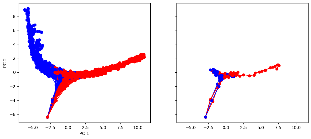
Transform individual trials and Visualize in PC space based on ground-truth color. We see that the neural activity is organized by stimulus ground-truth in PC1

plt.rcdefaults()
fig, (ax1, ax2) = plt.subplots(1, 2, sharey=True, sharex=True, figsize=(12, 5))
for i in range(num_trial):
    activity_pc = pca.transform(activity_dict[i])
    trial = trial_infos[i]
    color = 'red' if trial['ground_truth'] == 0 else 'blue'
    _ = ax1.plot(activity_pc[:, 0], activity_pc[:, 1], 'o-', color=color)
    if i < 5:
        _ = ax2.plot(activity_pc[:, 0], activity_pc[:, 1], 'o-', color=color)

ax1.set_xlabel('PC 1')
ax1.set_ylabel('PC 2')
plt.show()

Search for approximate fixed points

Here we search for approximate fixed points and visualize them in the same PC space. In a generic dynamical system,

\begin{align} \frac{d\mathbf{x}}{dt} = F(\mathbf{x}), \end{align}

We can search for fixed points by doing the optimization

\begin{align} \mathrm{argmin}_{\mathbf{x}} |F(\mathbf{x})|^2. \end{align}

f_cell = lambda h: net.cell(bm.asarray([1, 0.5, 0.5]), h)

fp_candidates = bm.vstack([activity_dict[i] for i in range(num_trial)])
fp_candidates.shape

(2200, 64)

finder = bp.analysis.SlowPointFinder(f_cell=f_cell, f_type='discrete')
finder.find_fps_with_gd_method(
  candidates=fp_candidates,
  tolerance=1e-5, num_batch=200,
    optimizer=bp.optim.Adam(lr=bp.optim.ExponentialDecay(0.01, 1, 0.9999)),
)
finder.filter_loss(tolerance=1e-5)
finder.keep_unique(tolerance=0.03)
finder.exclude_outliers(0.1)
fixed_points = finder.fixed_points

Optimizing with Adam(lr=ExponentialDecay(0.01, decay_steps=1, decay_rate=0.9999), last_call=-1), beta1=0.9, beta2=0.999, eps=1e-08) to find fixed points:
    Batches 1-200 in 0.74 sec, Training loss 0.0012789472
    Batches 201-400 in 0.69 sec, Training loss 0.0005247793
    Batches 401-600 in 0.68 sec, Training loss 0.0003411663
    Batches 601-800 in 0.69 sec, Training loss 0.0002612533
    Batches 801-1000 in 0.69 sec, Training loss 0.0002112046
    Batches 1001-1200 in 0.73 sec, Training loss 0.0001740992
    Batches 1201-1400 in 0.70 sec, Training loss 0.0001455246
    Batches 1401-1600 in 0.74 sec, Training loss 0.0001233126
    Batches 1601-1800 in 0.70 sec, Training loss 0.0001058684
    Batches 1801-2000 in 0.77 sec, Training loss 0.0000921902
    Batches 2001-2200 in 0.72 sec, Training loss 0.0000814899
    Batches 2201-2400 in 0.57 sec, Training loss 0.0000731918
    Batches 2401-2600 in 0.75 sec, Training loss 0.0000667152
    Batches 2601-2800 in 0.74 sec, Training loss 0.0000616670
    Batches 2801-3000 in 0.70 sec, Training loss 0.0000576638
    Batches 3001-3200 in 0.56 sec, Training loss 0.0000543614
    Batches 3201-3400 in 0.60 sec, Training loss 0.0000515535
    Batches 3401-3600 in 0.61 sec, Training loss 0.0000491180
    Batches 3601-3800 in 0.71 sec, Training loss 0.0000469084
    Batches 3801-4000 in 0.75 sec, Training loss 0.0000448209
    Batches 4001-4200 in 0.67 sec, Training loss 0.0000428211
    Batches 4201-4400 in 0.73 sec, Training loss 0.0000408868
    Batches 4401-4600 in 0.71 sec, Training loss 0.0000390110
    Batches 4601-4800 in 0.77 sec, Training loss 0.0000371877
    Batches 4801-5000 in 0.58 sec, Training loss 0.0000354225
    Batches 5001-5200 in 0.58 sec, Training loss 0.0000337130
    Batches 5201-5400 in 0.69 sec, Training loss 0.0000320665
    Batches 5401-5600 in 0.65 sec, Training loss 0.0000304907
    Batches 5601-5800 in 0.76 sec, Training loss 0.0000289806
    Batches 5801-6000 in 0.64 sec, Training loss 0.0000275472
    Batches 6001-6200 in 0.55 sec, Training loss 0.0000261840
    Batches 6201-6400 in 0.60 sec, Training loss 0.0000248957
    Batches 6401-6600 in 0.68 sec, Training loss 0.0000236831
    Batches 6601-6800 in 0.67 sec, Training loss 0.0000225569
    Batches 6801-7000 in 0.71 sec, Training loss 0.0000215175
    Batches 7001-7200 in 0.66 sec, Training loss 0.0000205547
    Batches 7201-7400 in 0.70 sec, Training loss 0.0000196768
    Batches 7401-7600 in 0.68 sec, Training loss 0.0000188892
    Batches 7601-7800 in 0.71 sec, Training loss 0.0000181973
    Batches 7801-8000 in 0.67 sec, Training loss 0.0000175776
    Batches 8001-8200 in 0.72 sec, Training loss 0.0000170112
    Batches 8201-8400 in 0.75 sec, Training loss 0.0000165215
    Batches 8401-8600 in 0.54 sec, Training loss 0.0000160938
    Batches 8601-8800 in 0.60 sec, Training loss 0.0000157249
    Batches 8801-9000 in 0.52 sec, Training loss 0.0000154070
    Batches 9001-9200 in 0.68 sec, Training loss 0.0000151405
    Batches 9201-9400 in 0.54 sec, Training loss 0.0000149151
    Batches 9401-9600 in 0.53 sec, Training loss 0.0000147287
    Batches 9601-9800 in 0.53 sec, Training loss 0.0000145786
    Batches 9801-10000 in 0.53 sec, Training loss 0.0000144657
Excluding fixed points with squared speed above tolerance 1e-05:
    Kept 1157/2200 fixed points with tolerance under 1e-05.
Excluding non-unique fixed points:
    Kept 10/1157 unique fixed points with uniqueness tolerance 0.03.
Excluding outliers:
    Kept 8/10 fixed points with within outlier tolerance 0.1.

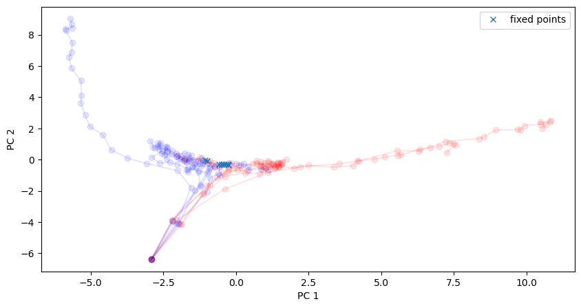
Visualize the found approximate fixed points.

We see that they found an approximate line attrator, corresponding to our PC1, along which evidence is integrated during the stimulus period.

# Plot in the same space as activity
plt.figure(figsize=(10, 5))
for i in range(10):
    activity_pc = pca.transform(activity_dict[i])
    trial = trial_infos[i]
    color = 'red' if trial['ground_truth'] == 0 else 'blue'
    plt.plot(activity_pc[:, 0], activity_pc[:, 1], 'o-', color=color, alpha=0.1)

# Fixed points are shown in cross
fixedpoints_pc = pca.transform(fixed_points)
plt.plot(fixedpoints_pc[:, 0], fixedpoints_pc[:, 1], 'x', label='fixed points')

plt.xlabel('PC 1')
plt.ylabel('PC 2')
plt.legend()
plt.show()

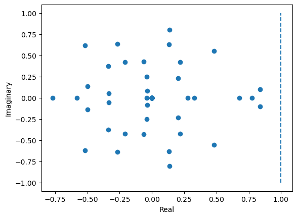
Computing the Jacobian and finding the line attractor

from jax import jacobian

dFdh = jacobian(f_cell)(fixed_points[2])

eigval, eigvec = np.linalg.eig(bm.as_numpy(dFdh))

# Plot distribution of eigenvalues in a 2-d real-imaginary plot
plt.figure()
plt.scatter(np.real(eigval), np.imag(eigval))
plt.plot([1, 1], [-1, 1], '--')
plt.xlabel('Real')
plt.ylabel('Imaginary')
plt.show()