(Vreeswijk & Sompolinsky, 1996) E/I balanced network

Overviews

Van Vreeswijk and Sompolinsky proposed E-I balanced network in 1996 to explain the temporally irregular spiking patterns. They suggested that the temporal variability may originated from the balance between excitatory and inhibitory inputs.

There are \(N_E\) excitatory neurons and \(N_I\) inbibitory neurons.

An important feature of the network is random and sparse connectivity. Connections between neurons \(K\) meets \(1 << K << N_E\).

Implementations

[13]:

import brainpy as bp
import brainpy.math as bm

bm.set_platform('cpu')

[14]:

bp.__version__

[14]:

'2.4.4.post1'

Dynamic of membrane potential is given as:

\[\tau \frac {dV_i}{dt} = -(V_i - V_{rest}) + I_i^{ext} + I_i^{net} (t)\]

where \(I_i^{net}(t)\) represents the synaptic current, which describes the sum of excitatory and inhibitory neurons.

\[I_i^{net} (t) = J_E \sum_{j=1}^{pN_e} \sum_{t_j^\alpha < t} f(t-t_j^\alpha ) - J_I \sum_{j=1}^{pN_i} \sum_{t_j^\alpha < t} f(t-t_j^\alpha )\]

where

\[\begin{split} f(t) = \begin{cases} {\rm exp} (-\frac t {\tau_s} ), \quad t \geq 0 \\ 0, \quad t < 0 \end{cases}\end{split}\]

Parameters: \(J_E = \frac 1 {\sqrt {pN_e}}, J_I = \frac 1 {\sqrt {pN_i}}\)

We can see from the dynamic that network is based on leaky Integrate-and-Fire neurons, and we can just use get_LIF from bpmodels.neurons to get this model.

The function of \(I_i^{net}(t)\) is actually a synase with single exponential decay, we can also get it by using get_exponential.

Synapse

[15]:

class ExponCUBA(bp.Projection):
    def __init__(self, pre, post, prob, g_max, tau):
        super().__init__()
        self.proj = bp.dyn.ProjAlignPostMg2(
            pre=pre,
            delay=None,
            comm=bp.dnn.EventCSRLinear(bp.conn.FixedProb(prob, pre=pre.num, post=post.num), g_max),
            syn=bp.dyn.Expon.desc(post.num, tau=tau),
            out=bp.dyn.CUBA.desc(),
            post=post,
        )

Network

Let’s create a neuron group with \(N_E\) excitatory neurons and \(N_I\) inbibitory neurons. Use conn=bp.connect.FixedProb(p) to implement the random and sparse connections.

[16]:

class EINet(bp.DynSysGroup):
  def __init__(self, num_exc, num_inh, prob, JE, JI):
    # neurons
    pars = dict(V_rest=-52., V_th=-50., V_reset=-60., tau=10., tau_ref=0.,
                V_initializer=bp.init.Normal(-60., 10.))
    E = bp.neurons.LIF(num_exc, **pars)
    I = bp.neurons.LIF(num_inh, **pars)

    # synapses
    E2E = ExponCUBA(E, E, prob, g_max=JE, tau=2.)
    E2I = ExponCUBA(E, I, prob, g_max=JE, tau=2.)
    I2E = ExponCUBA(I, E, prob, g_max=JI, tau=2.)
    I2I = ExponCUBA(I, I, prob, g_max=JI, tau=2.)

    super(EINet, self).__init__(E2E, E2I, I2E, I2I, E=E, I=I)

[17]:

num_exc = 500
num_inh = 500
prob = 0.1

Ib = 3.
JE = 1 / bp.math.sqrt(prob * num_exc)
JI = -1 / bp.math.sqrt(prob * num_inh)

[18]:

net = EINet(num_exc, num_inh, prob=prob, JE=JE, JI=JI)

runner = bp.DSRunner(net,
                     monitors=['E.spike'],
                     inputs=[('E.input', Ib), ('I.input', Ib)])
t = runner.run(1000.)

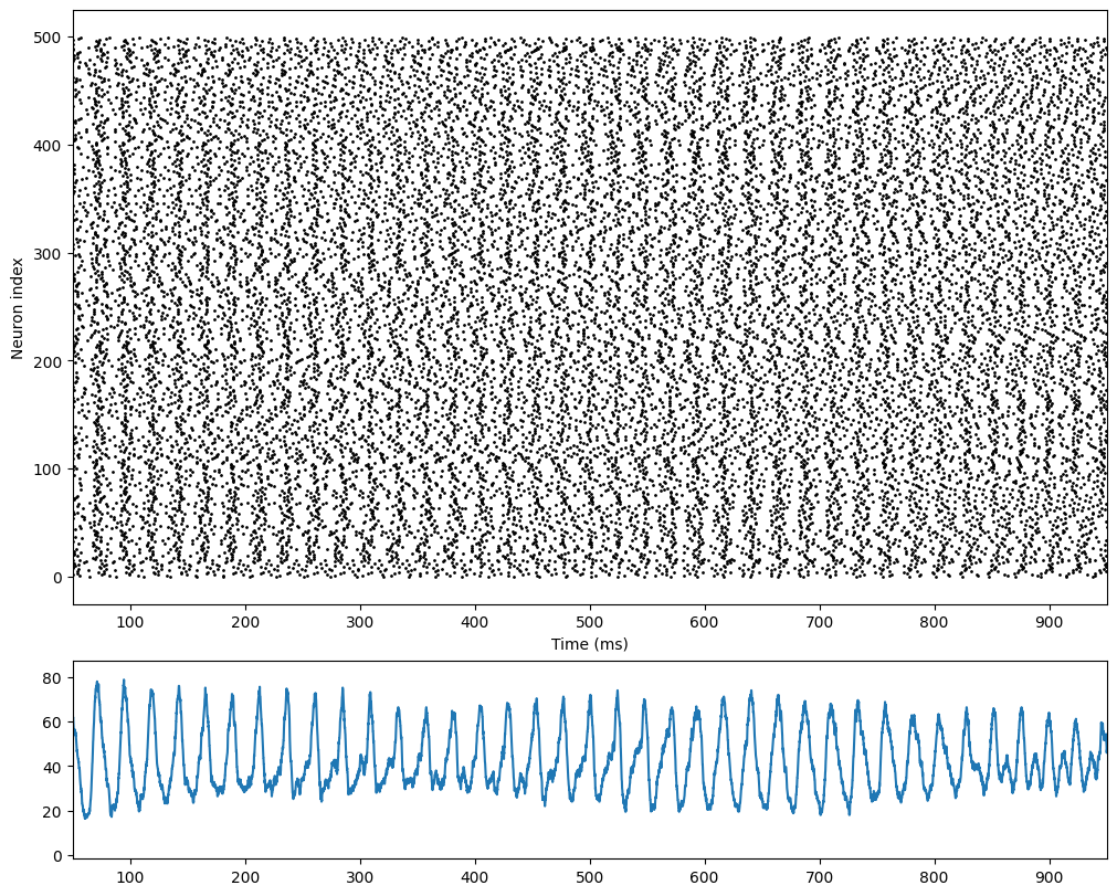
Visualization

[19]:

import matplotlib.pyplot as plt

fig, gs = bp.visualize.get_figure(4, 1, 2, 10)

fig.add_subplot(gs[:3, 0])
bp.visualize.raster_plot(runner.mon.ts, runner.mon['E.spike'], xlim=(50, 950))

fig.add_subplot(gs[3, 0])
rates = bp.measure.firing_rate(runner.mon['E.spike'], 5.)
plt.plot(runner.mon.ts, rates)
plt.xlim(50, 950)
plt.show()

../_images/ei_nets_Vreeswijk_1996_EI_net_17_0.png

Reference

[1] Van Vreeswijk, Carl, and Haim Sompolinsky. “Chaos in neuronal networks with balanced excitatory and inhibitory activity.” Science 274.5293 (1996): 1724-1726.