(Niebur, et. al, 2009) Generalized integrate-and-fire model

Implementation of the paper: Mihalaş, Ştefan, and Ernst Niebur. “A generalized linear integrate-and-fire neural model produces diverse spiking behaviors.” Neural computation 21.3 (2009): 704-718.

[1]:

import matplotlib.pyplot as plt
import brainpy as bp

Model Overview

Generalized integrate-and-fire model is a spiking neuron model, describes single neuron behavior and can generate most kinds of firing patterns by tuning parameters.

Generalized IF model is originated from Leaky Integrate-and-Fire model (LIF model), yet it’s differentiated from LIF model, for it includes internal currents \(I_j\) in its expressions.

\[\frac{d I_j}{d t} = -k_j I_j\]

\[\tau\frac{d V}{d t} = - (V - V_{rest}) + R\sum_{j}I_j + RI\]

\[\frac{d V_{th}}{d t} = a(V - V_{rest}) - b(V_{th} - V_{th\infty})\]

Generalized IF neuron fire when \(V\) meet \(V_{th}\):

\[I_j \leftarrow R_j I_j + A_j\]

\[V \leftarrow V_{reset}\]

\[V_{th} \leftarrow max(V_{th_{reset}}, V_{th})\]

Different firing patterns

These arbitrary number of internal currents \(I_j\) can be seen as currents caused by ion channels’ dynamics, provides the GeneralizedIF model a flexibility to generate various firing patterns.

With appropriate parameters, we can reproduce most of the single neuron firing patterns. In the original paper (Mihalaş et al., 2009), the author used two internal currents \(I1\) and \(I2\).

[2]:

def run(model, duration, I_ext):
  runner = bp.DSRunner(model,
                       inputs=('input', I_ext, 'iter'),
                       monitors=['V', 'V_th'])
  runner.run(duration)

  ts = runner.mon.ts
  fig, gs = bp.visualize.get_figure(1, 1, 4, 8)
  ax1 = fig.add_subplot(gs[0, 0])
  #ax1.title.set_text(f'{mode}')

  ax1.plot(ts, runner.mon.V[:, 0], label='V')
  ax1.plot(ts, runner.mon.V_th[:, 0], label='V_th')
  ax1.set_xlabel('Time (ms)')
  ax1.set_ylabel('Membrane potential')
  ax1.set_xlim(-0.1, ts[-1] + 0.1)
  plt.legend()

  ax2 = ax1.twinx()
  ax2.plot(ts, I_ext, color='turquoise', label='input')
  ax2.set_xlabel('Time (ms)')
  ax2.set_ylabel('External input')
  ax2.set_xlim(-0.1, ts[-1] + 0.1)
  ax2.set_ylim(-5., 20.)
  plt.legend(loc='lower left')
  plt.show()

Simulate Generalized IF neuron groups to generate different spiking patterns. Here we plot 20 spiking patterns in groups of 4. The plots are labeled with corresponding pattern names above the plots.

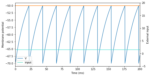
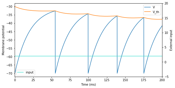
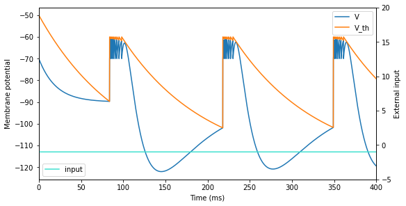
Tonic Spiking

[3]:

Iext, duration = bp.inputs.constant_input([(1.5, 200.)])
neu = bp.neurons.GIF(1)
run(neu, duration, Iext)

WARNING:jax._src.lib.xla_bridge:No GPU/TPU found, falling back to CPU. (Set TF_CPP_MIN_LOG_LEVEL=0 and rerun for more info.)

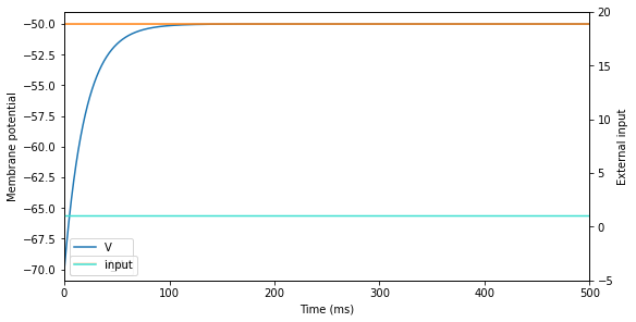
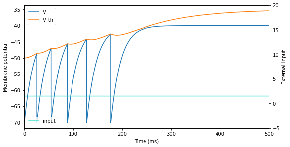
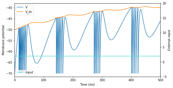
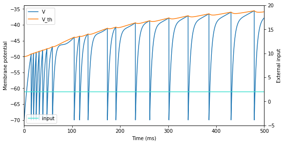
../_images/neurons_Niebur_2009_GIF_13_2.png

Class 1 Excitability

[4]:

Iext, duration = bp.inputs.constant_input([(1. + 1e-6, 500.)])
neu = bp.neurons.GIF(1)
run(neu, duration, Iext)

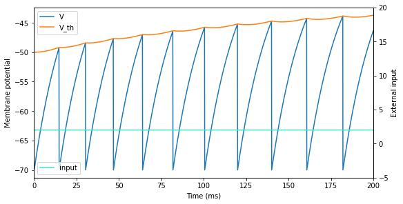
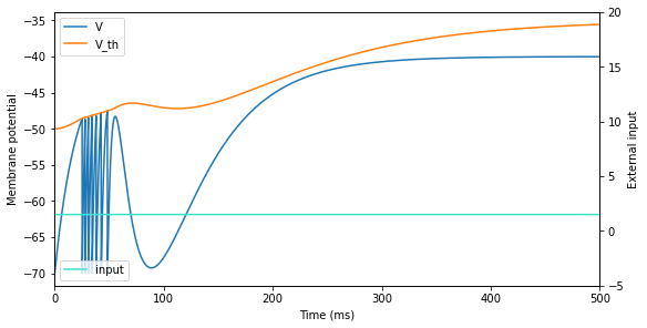
../_images/neurons_Niebur_2009_GIF_15_1.png

Spike Frequency Adaptation

[5]:

Iext, duration = bp.inputs.constant_input([(2., 200.)])
neu = bp.neurons.GIF(1, a=0.005)
run(neu, duration, Iext)

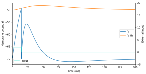
../_images/neurons_Niebur_2009_GIF_17_1.png

Phasic Spiking

[6]:

Iext, duration = bp.inputs.constant_input([(1.5, 500.)])
neu = bp.neurons.GIF(1, a=0.005)
run(neu, duration, Iext)

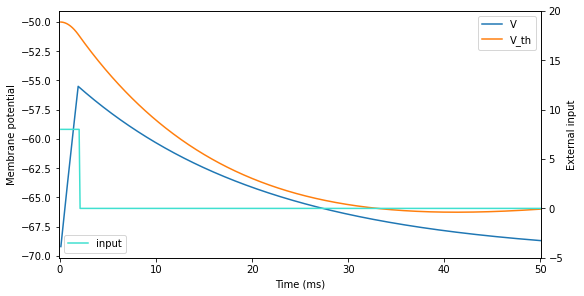
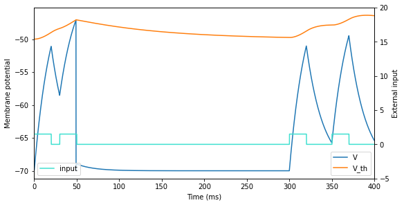
../_images/neurons_Niebur_2009_GIF_19_1.png

Accomodation

[7]:

Iext, duration = bp.inputs.constant_input([(1.5, 100.),
                                           (0, 500.),
                                           (0.5, 100.),
                                           (1., 100.),
                                           (1.5, 100.),
                                           (0., 100.)])
neu = bp.neurons.GIF(1, a=0.005)
run(neu, duration, Iext)

../_images/neurons_Niebur_2009_GIF_21_1.png

Threshold Variability

[8]:

Iext, duration = bp.inputs.constant_input([(1.5, 20.),
                                           (0., 180.),
                                           (-1.5, 20.),
                                           (0., 20.),
                                           (1.5, 20.),
                                           (0., 140.)])
neu = bp.neurons.GIF(1, a=0.005)
run(neu, duration, Iext)

../_images/neurons_Niebur_2009_GIF_23_1.png

Rebound Spiking

[9]:

Iext, duration = bp.inputs.constant_input([(0, 50.), (-3.5, 750.), (0., 200.)])
neu = bp.neurons.GIF(1, a=0.005)
run(neu, duration, Iext)

../_images/neurons_Niebur_2009_GIF_25_1.png

Class 2 Excitability

[10]:

Iext, duration = bp.inputs.constant_input([(2 * (1. + 1e-6), 200.)])
neu = bp.neurons.GIF(1, a=0.005)
neu.V_th[:] = -30.
run(neu, duration, Iext)

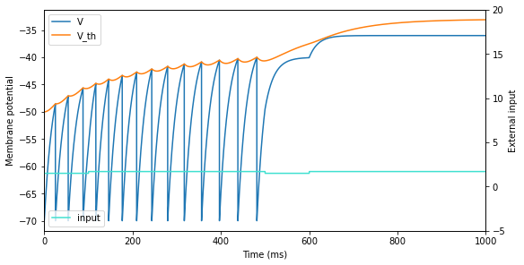
../_images/neurons_Niebur_2009_GIF_27_1.png

Integrator

[11]:

Iext, duration = bp.inputs.constant_input([(1.5, 20.),
                                           (0., 10.),
                                           (1.5, 20.),
                                           (0., 250.),
                                           (1.5, 20.),
                                           (0., 30.),
                                           (1.5, 20.),
                                           (0., 30.)])
neu = bp.neurons.GIF(1, a=0.005)
run(neu, duration, Iext)

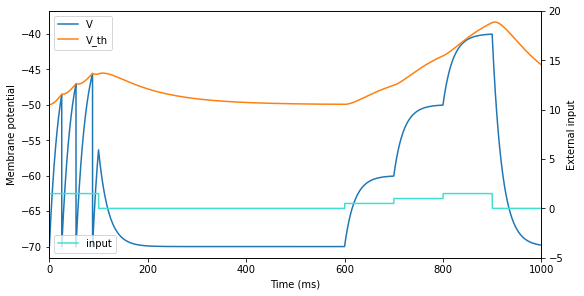
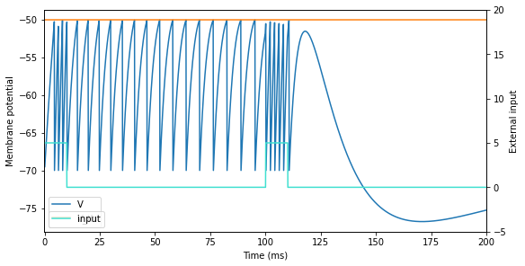
../_images/neurons_Niebur_2009_GIF_29_1.png

Input Bistability

[12]:

Iext, duration = bp.inputs.constant_input([(1.5, 100.),
                                           (1.7, 400.),
                                           (1.5, 100.),
                                           (1.7, 400.)])
neu = bp.neurons.GIF(1, a=0.005)
run(neu, duration, Iext)

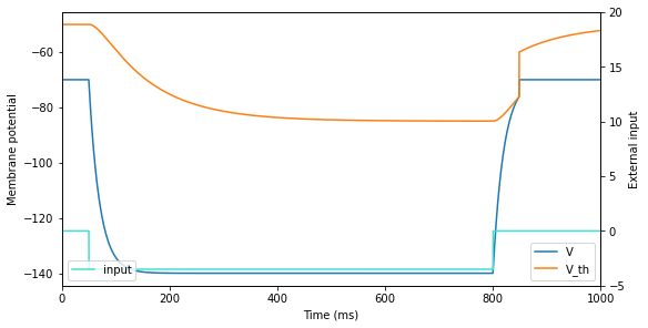
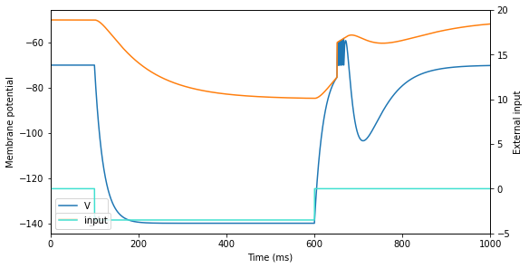
../_images/neurons_Niebur_2009_GIF_31_1.png

Hyperpolarization-induced Spiking

[13]:

Iext, duration = bp.inputs.constant_input([(-1., 400.)])
neu = bp.neurons.GIF(1, V_th_reset=-60., V_th_inf=-120.)
neu.V_th[:] = -50.
run(neu, duration, Iext)

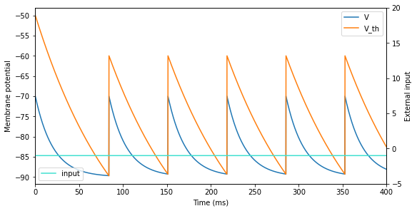
../_images/neurons_Niebur_2009_GIF_33_1.png

Hyperpolarization-induced Bursting

[14]:

Iext, duration = bp.inputs.constant_input([(-1., 400.)])
neu = bp.neurons.GIF(1, V_th_reset=-60., V_th_inf=-120., A1=10.,
                 A2=-0.6)
neu.V_th[:] = -50.
run(neu, duration, Iext)

../_images/neurons_Niebur_2009_GIF_35_1.png

Tonic Bursting

[15]:

Iext, duration = bp.inputs.constant_input([(2., 500.)])
neu = bp.neurons.GIF(1, a=0.005, A1=10., A2=-0.6)
run(neu, duration, Iext)

../_images/neurons_Niebur_2009_GIF_37_1.png

Phasic Bursting

[16]:

Iext, duration = bp.inputs.constant_input([(1.5, 500.)])
neu = bp.neurons.GIF(1, a=0.005, A1=10., A2=-0.6)
run(neu, duration, Iext)

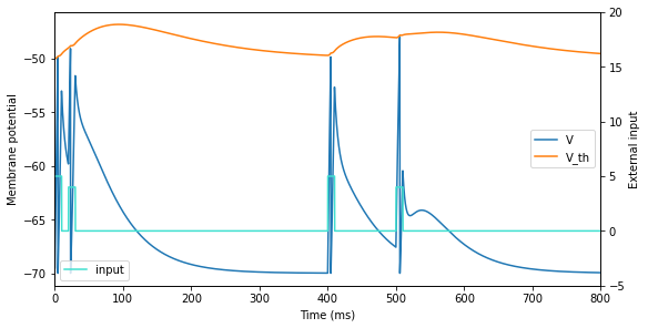
../_images/neurons_Niebur_2009_GIF_39_1.png

Rebound Bursting

[17]:

Iext, duration = bp.inputs.constant_input([(0, 100.), (-3.5, 500.), (0., 400.)])
neu = bp.neurons.GIF(1, a=0.005, A1=10., A2=-0.6)
run(neu, duration, Iext)

../_images/neurons_Niebur_2009_GIF_41_1.png

Mixed Mode

[18]:

Iext, duration = bp.inputs.constant_input([(2., 500.)])
neu = bp.neurons.GIF(1, a=0.005, A1=5., A2=-0.3)
run(neu, duration, Iext)

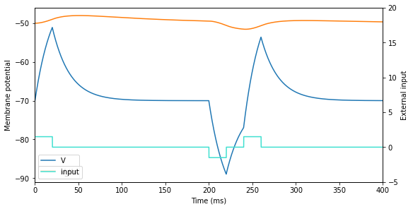
../_images/neurons_Niebur_2009_GIF_43_1.png

Afterpotentials

[19]:

Iext, duration = bp.inputs.constant_input([(2., 15.), (0, 185.)])
neu = bp.neurons.GIF(1, a=0.005, A1=5., A2=-0.3)
run(neu, duration, Iext)

../_images/neurons_Niebur_2009_GIF_45_1.png

Basal Bistability

[20]:

Iext, duration = bp.inputs.constant_input([(5., 10.), (0., 90.), (5., 10.), (0., 90.)])
neu = bp.neurons.GIF(1, A1=8., A2=-0.1)
run(neu, duration, Iext)

../_images/neurons_Niebur_2009_GIF_47_1.png

Preferred Frequency

[21]:

Iext, duration = bp.inputs.constant_input([(5., 10.),
                                           (0., 10.),
                                           (4., 10.),
                                           (0., 370.),
                                           (5., 10.),
                                           (0., 90.),
                                           (4., 10.),
                                           (0., 290.)])
neu = bp.neurons.GIF(1, a=0.005, A1=-3., A2=0.5)
run(neu, duration, Iext)

../_images/neurons_Niebur_2009_GIF_49_1.png

Spike Latency

[22]:

Iext, duration = bp.inputs.constant_input([(8., 2.), (0, 48.)])
neu = bp.neurons.GIF(1, a=-0.08)
run(neu, duration, Iext)

../_images/neurons_Niebur_2009_GIF_51_1.png