(Gauthier, et. al, 2021): Next generation reservoir computing
![]()

Implementation of the paper:
Gauthier, D.J., Bollt, E., Griffith, A. et al. Next generation reservoir computing. Nat Commun 12, 5564 (2021). https://doi.org/10.1038/s41467-021-25801-2
[27]:
import matplotlib.pyplot as plt
import numpy as np

import brainpy as bp
import brainpy.math as bm
import brainpy_datasets as bd

bm.set(mode=bm.batching_mode, x64=True)
[28]:
bp.__version__
[28]:
'2.4.3'
[29]:
def plot_weights(Wout, coefs, bias=None):
  Wout = np.asarray(Wout)
  if bias is not None:
    bias = np.asarray(bias)
    Wout = np.concatenate([bias.reshape((1, 3)), Wout], axis=0)
    coefs.insert(0, 'bias')
  x_Wout, y_Wout, z_Wout = Wout[:, 0], Wout[:, 1], Wout[:, 2]

  fig = plt.figure(figsize=(10, 10))
  ax = fig.add_subplot(131)
  ax.grid(axis="y")
  ax.set_xlabel("$[W_{out}]_x$")
  ax.set_ylabel("Features")
  ax.set_yticks(np.arange(len(coefs)))
  ax.set_yticklabels(coefs)
  ax.barh(np.arange(x_Wout.size), x_Wout)

  ax1 = fig.add_subplot(132)
  ax1.grid(axis="y")
  ax1.set_yticks(np.arange(len(coefs)))
  ax1.set_xlabel("$[W_{out}]_y$")
  ax1.barh(np.arange(y_Wout.size), y_Wout)

  ax2 = fig.add_subplot(133)
  ax2.grid(axis="y")
  ax2.set_yticks(np.arange(len(coefs)))
  ax2.set_xlabel("$[W_{out}]_z$")
  ax2.barh(np.arange(z_Wout.size), z_Wout)

  plt.show()
Forecasting Lorenz63 strange attractor
[30]:
def get_subset(data, start, end):
  res = {'x': data.xs[start: end],
         'y': data.ys[start: end],
         'z': data.zs[start: end]}
  res = bm.hstack([res['x'], res['y'], res['z']])
  return res.reshape((1, ) + res.shape)
[31]:
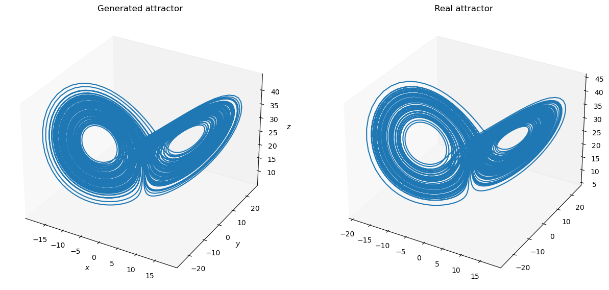
def plot_lorenz(ground_truth, predictions):
  fig = plt.figure(figsize=(15, 10))
  ax = fig.add_subplot(121, projection='3d')
  ax.set_title("Generated attractor")
  ax.set_xlabel("$x$")
  ax.set_ylabel("$y$")
  ax.set_zlabel("$z$")
  ax.grid(False)
  ax.plot(predictions[:, 0], predictions[:, 1], predictions[:, 2])

  ax2 = fig.add_subplot(122, projection='3d')
  ax2.set_title("Real attractor")
  ax2.grid(False)
  ax2.plot(ground_truth[:, 0], ground_truth[:, 1], ground_truth[:, 2])
  plt.show()
[32]:
dt = 0.01
t_warmup = 5.  # ms
t_train = 10.  # ms
t_test = 120.  # ms
num_warmup = int(t_warmup / dt)  # warm up NVAR
num_train = int(t_train / dt)
num_test = int(t_test / dt)
Datasets
[33]:
lorenz_series = bd.chaos.LorenzEq(t_warmup + t_train + t_test,
                                  dt=dt,
                                  inits={'x': 17.67715816276679,
                                         'y': 12.931379185960404,
                                         'z': 43.91404334248268})

X_warmup = get_subset(lorenz_series, 0, num_warmup - 1)
Y_warmup = get_subset(lorenz_series, 1, num_warmup)
X_train = get_subset(lorenz_series, num_warmup - 1, num_warmup + num_train - 1)
# Target: Lorenz[t] - Lorenz[t - 1]
dX_train = get_subset(lorenz_series, num_warmup, num_warmup + num_train) - X_train
X_test = get_subset(lorenz_series,
                    num_warmup + num_train - 1,
                    num_warmup + num_train + num_test - 1)
Y_test = get_subset(lorenz_series,
                    num_warmup + num_train,
                    num_warmup + num_train + num_test)
Model
[34]:
class NGRC(bp.DynamicalSystem):
  def __init__(self, num_in):
    super(NGRC, self).__init__()
    self.r = bp.dyn.NVAR(num_in, delay=2, order=2, constant=True,)
    self.di = bp.dnn.Dense(self.r.num_out, num_in, b_initializer=None, mode=bm.training_mode)

  def update(self, x):
    dx = self.di(self.r(x))
    return x + dx
[35]:
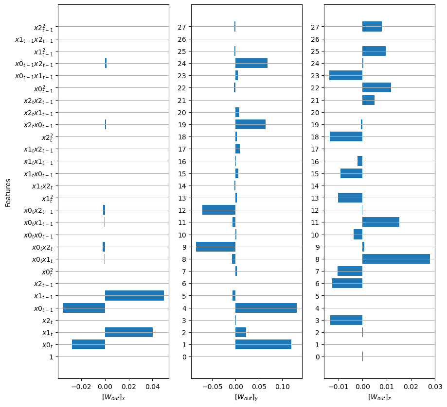
model = NGRC(3)
print(model.r.get_feature_names())
['1', 'x0(t)', 'x1(t)', 'x2(t)', 'x0(t-1)', 'x1(t-1)', 'x2(t-1)', 'x0(t)^2', 'x0(t) x1(t)', 'x0(t) x2(t)', 'x0(t) x0(t-1)', 'x0(t) x1(t-1)', 'x0(t) x2(t-1)', 'x1(t)^2', 'x1(t) x2(t)', 'x1(t) x0(t-1)', 'x1(t) x1(t-1)', 'x1(t) x2(t-1)', 'x2(t)^2', 'x2(t) x0(t-1)', 'x2(t) x1(t-1)', 'x2(t) x2(t-1)', 'x0(t-1)^2', 'x0(t-1) x1(t-1)', 'x0(t-1) x2(t-1)', 'x1(t-1)^2', 'x1(t-1) x2(t-1)', 'x2(t-1)^2']
Training
[36]:
# warm-up
trainer = bp.RidgeTrainer(model, alpha=2.5e-6)

# training
outputs = trainer.predict(X_warmup)
print('Warmup NMS: ', bp.losses.mean_squared_error(outputs, Y_warmup))
trainer.fit([X_train, dX_train])
plot_weights(model.di.W, model.r.get_feature_names(for_plot=True), model.di.b)
Warmup NMS: 69547.9569984571
Prediction
[37]:
model = bm.jit(model)
outputs = [model(dict(), X_test[:, 0])]
for i in range(1, X_test.shape[1]):
  outputs.append(model(dict(), outputs[i - 1]))
outputs = bm.asarray(outputs)
print('Prediction NMS: ', bp.losses.mean_squared_error(outputs, Y_test))
plot_lorenz(bm.as_numpy(Y_test).squeeze(), bm.as_numpy(outputs).squeeze())
Prediction NMS: 148.18244150701176
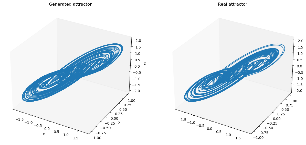
Forecasting the double-scroll system
[38]:
def plot_double_scroll(ground_truth, predictions):
  fig = plt.figure(figsize=(15, 10))
  ax = fig.add_subplot(121, projection='3d')
  ax.set_title("Generated attractor")
  ax.set_xlabel("$x$")
  ax.set_ylabel("$y$")
  ax.set_zlabel("$z$")
  ax.grid(False)
  ax.plot(predictions[:, 0], predictions[:, 1], predictions[:, 2])

  ax2 = fig.add_subplot(122, projection='3d')
  ax2.set_title("Real attractor")
  ax2.grid(False)
  ax2.plot(ground_truth[:, 0], ground_truth[:, 1], ground_truth[:, 2])
  plt.show()
[39]:
dt = 0.02
t_warmup = 10.  # ms
t_train = 100.  # ms
t_test = 800.  # ms
num_warmup = int(t_warmup / dt)  # warm up NVAR
num_train = int(t_train / dt)
num_test = int(t_test / dt)
Datasets
[40]:
data_series = bd.chaos.DoubleScrollEq(t_warmup + t_train + t_test, dt=dt)

X_warmup = get_subset(data_series, 0, num_warmup - 1)
Y_warmup = get_subset(data_series, 1, num_warmup)
X_train = get_subset(data_series, num_warmup - 1, num_warmup + num_train - 1)
# Target: Lorenz[t] - Lorenz[t - 1]
dX_train = get_subset(data_series, num_warmup, num_warmup + num_train) - X_train
X_test = get_subset(data_series,
                    num_warmup + num_train - 1,
                    num_warmup + num_train + num_test - 1)
Y_test = get_subset(data_series,
                    num_warmup + num_train,
                    num_warmup + num_train + num_test)
Model
[41]:
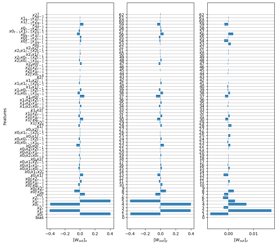
class NGRC(bp.DynamicalSystem):
  def __init__(self, num_in):
    super().__init__()
    self.r = bp.dyn.NVAR(num_in, delay=2, order=3)
    self.di = bp.dnn.Dense(self.r.num_out, num_in, mode=bm.training_mode)

  def update(self, x):
    di = self.di(self.r(x))
    return x + di

model = NGRC(3)
Training
[42]:
# warm-up
trainer = bp.RidgeTrainer(model, alpha=1e-5, jit=True)
[43]:
# training
outputs = trainer.predict(X_warmup)
print('Warmup NMS: ', bp.losses.mean_squared_error(outputs, Y_warmup))
trainer.fit([X_train, dX_train])
plot_weights(model.di.W, model.r.get_feature_names(for_plot=True), model.di.b)
Warmup NMS: 3.8119375651557474
Prediction
[44]:
model = bm.jit(model)
outputs = [model(dict(), X_test[:, 0])]
for i in range(1, X_test.shape[1]):
  outputs.append(model(dict(), outputs[i - 1]))
outputs = bm.asarray(outputs).squeeze()
print('Prediction NMS: ', bp.losses.mean_squared_error(outputs, Y_test))
plot_double_scroll(Y_test.numpy().squeeze(), outputs.numpy())
Prediction NMS: 1.795131408515274
Infering dynamics of Lorenz63 strange attractor
[45]:
def get_subset(data, start, end):
  res = {'x': data.xs[start: end],
         'y': data.ys[start: end],
         'z': data.zs[start: end]}
  X = bm.hstack([res['x'], res['y']])
  X = X.reshape((1,) + X.shape)
  Y = res['z']
  Y = Y.reshape((1, ) + Y.shape)
  return X, Y
[46]:
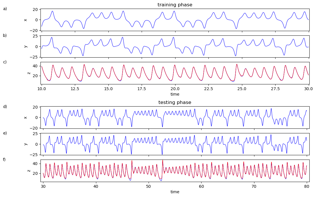
def plot_lorenz2(x, y, true_z, predict_z, linewidth=.8):
  fig1 = plt.figure()
  fig1.set_figheight(8)
  fig1.set_figwidth(12)

  t_all = t_warmup + t_train + t_test
  ts = np.arange(0, t_all, dt)

  h = 240
  w = 2

  # top left of grid is 0,0
  axs1 = plt.subplot2grid(shape=(h, w), loc=(0, 0), colspan=2, rowspan=30)
  axs2 = plt.subplot2grid(shape=(h, w), loc=(36, 0), colspan=2, rowspan=30)
  axs3 = plt.subplot2grid(shape=(h, w), loc=(72, 0), colspan=2, rowspan=30)
  axs4 = plt.subplot2grid(shape=(h, w), loc=(132, 0), colspan=2, rowspan=30)
  axs5 = plt.subplot2grid(shape=(h, w), loc=(168, 0), colspan=2, rowspan=30)
  axs6 = plt.subplot2grid(shape=(h, w), loc=(204, 0), colspan=2, rowspan=30)

  # training phase x
  axs1.set_title('training phase')
  axs1.plot(ts[num_warmup:num_warmup + num_train],
            x[num_warmup:num_warmup + num_train],
            color='b', linewidth=linewidth)
  axs1.set_ylabel('x')
  axs1.axes.xaxis.set_ticklabels([])
  axs1.axes.set_xbound(t_warmup - .08, t_warmup + t_train + .05)
  axs1.axes.set_ybound(-21., 21.)
  axs1.text(-.14, .9, 'a)', ha='left', va='bottom', transform=axs1.transAxes)

  # training phase y
  axs2.plot(ts[num_warmup:num_warmup + num_train],
            y[num_warmup:num_warmup + num_train],
            color='b', linewidth=linewidth)
  axs2.set_ylabel('y')
  axs2.axes.xaxis.set_ticklabels([])
  axs2.axes.set_xbound(t_warmup - .08, t_warmup + t_train + .05)
  axs2.axes.set_ybound(-26., 26.)
  axs2.text(-.14, .9, 'b)', ha='left', va='bottom', transform=axs2.transAxes)

  # training phase z
  axs3.plot(ts[num_warmup:num_warmup + num_train],
            true_z[num_warmup:num_warmup + num_train],
            color='b', linewidth=linewidth)
  axs3.plot(ts[num_warmup:num_warmup + num_train],
            predict_z[num_warmup:num_warmup + num_train],
            color='r', linewidth=linewidth)
  axs3.set_ylabel('z')
  axs3.set_xlabel('time')
  axs3.axes.set_xbound(t_warmup - .08, t_warmup + t_train + .05)
  axs3.axes.set_ybound(3., 48.)
  axs3.text(-.14, .9, 'c)', ha='left', va='bottom', transform=axs3.transAxes)

  # testing phase x
  axs4.set_title('testing phase')
  axs4.plot(ts[num_warmup + num_train:num_warmup + num_train + num_test],
            x[num_warmup + num_train:num_warmup + num_train + num_test],
            color='b', linewidth=linewidth)
  axs4.set_ylabel('x')
  axs4.axes.xaxis.set_ticklabels([])
  axs4.axes.set_ybound(-21., 21.)
  axs4.axes.set_xbound(t_warmup + t_train - .5, t_all + .5)
  axs4.text(-.14, .9, 'd)', ha='left', va='bottom', transform=axs4.transAxes)

  # testing phase y
  axs5.plot(ts[num_warmup + num_train:num_warmup + num_train + num_test],
            y[num_warmup + num_train:num_warmup + num_train + num_test],
            color='b', linewidth=linewidth)
  axs5.set_ylabel('y')
  axs5.axes.xaxis.set_ticklabels([])
  axs5.axes.set_ybound(-26., 26.)
  axs5.axes.set_xbound(t_warmup + t_train - .5, t_all + .5)
  axs5.text(-.14, .9, 'e)', ha='left', va='bottom', transform=axs5.transAxes)

  # testing phose z
  axs6.plot(ts[num_warmup + num_train:num_warmup + num_train + num_test],
            true_z[num_warmup + num_train:num_warmup + num_train + num_test],
            color='b', linewidth=linewidth)
  axs6.plot(ts[num_warmup + num_train:num_warmup + num_train + num_test],
            predict_z[num_warmup + num_train:num_warmup + num_train + num_test],
            color='r', linewidth=linewidth)
  axs6.set_ylabel('z')
  axs6.set_xlabel('time')
  axs6.axes.set_ybound(3., 48.)
  axs6.axes.set_xbound(t_warmup + t_train - .5, t_all + .5)
  axs6.text(-.14, .9, 'f)', ha='left', va='bottom', transform=axs6.transAxes)

  plt.show()
[47]:
dt = 0.02
t_warmup = 10.  # ms
t_train = 20.  # ms
t_test = 50.  # ms
num_warmup = int(t_warmup / dt)  # warm up NVAR
num_train = int(t_train / dt)
num_test = int(t_test / dt)
Datasets
[48]:
lorenz_series = bd.chaos.LorenzEq(t_warmup + t_train + t_test,
                                  dt=dt,
                                  inits={'x': 17.67715816276679,
                                         'y': 12.931379185960404,
                                         'z': 43.91404334248268})

X_warmup, Y_warmup = get_subset(lorenz_series, 0, num_warmup)
X_train, Y_train = get_subset(lorenz_series, num_warmup, num_warmup + num_train)
X_test, Y_test = get_subset(lorenz_series, 0, num_warmup + num_train + num_test)
Model
[49]:
class NGRC(bp.DynamicalSystem):
  def __init__(self, num_in):
    super().__init__()
    self.r = bp.dyn.NVAR(num_in, delay=4, order=2, stride=5)
    self.o = bp.dnn.Dense(self.r.num_out, 1, mode=bm.training_mode)

  def update(self, x):
    return self.o(self.r(x))


model = NGRC(2)
Training
[50]:
trainer = bp.RidgeTrainer(model, alpha=0.05)

# warm-up
outputs = trainer.predict(X_warmup)
print('Warmup NMS: ', bp.losses.mean_squared_error(outputs, Y_warmup))

# training
_ = trainer.fit([X_train, Y_train])
Warmup NMS: 52397.382810820985
Prediction
[51]:
outputs = trainer.predict(X_test, reset_state=True)
print('Prediction NMS: ', bp.losses.mean_squared_error(outputs, Y_test))
Prediction NMS: 590.5516566499861
[52]:
plot_lorenz2(x=bm.as_numpy(lorenz_series.xs.flatten()),
             y=bm.as_numpy(lorenz_series.ys.flatten()),
             true_z=bm.as_numpy(lorenz_series.zs.flatten()),
             predict_z=bm.as_numpy(outputs.flatten()))