(Song, et al., 2016): Training excitatory-inhibitory recurrent network

Implementation of the paper:

• Song, H. F. , G. R. Yang , and X. J. Wang . “Training Excitatory-Inhibitory Recurrent Neural Networks for Cognitive Tasks: A Simple and Flexible Framework.” Plos Computational Biology 12.2(2016):e1004792.

The original code is based on PyTorch (https://github.com/gyyang/nn-brain/blob/master/EI_RNN.ipynb). However, comparing with the PyTorch codes, the training on BrainPy speeds up nearly four folds.

Here we will train recurrent neural network with excitatory and inhibitory neurons on a simple perceptual decision making task.

import brainpy as bp
import brainpy.math as bm
bp.math.set_platform('cpu')

import numpy as np
import matplotlib.pyplot as plt

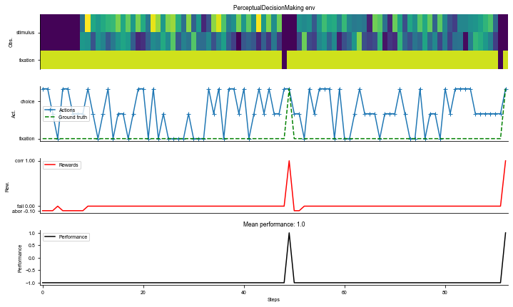
Defining a perceptual decision making task

# We will import the task from the neurogym library.
# Please install neurogym:
#
# https://github.com/neurogym/neurogym

import neurogym as ngym

# Environment
task = 'PerceptualDecisionMaking-v0'
timing = {
  'fixation': ('choice', (50, 100, 200, 400)),
  'stimulus': ('choice', (100, 200, 400, 800)),
}
kwargs = {'dt': 20, 'timing': timing}
seq_len = 100

# Make supervised dataset
dataset = ngym.Dataset(task,
                       env_kwargs=kwargs,
                       batch_size=16,
                       seq_len=seq_len)

# A sample environment from dataset
env = dataset.env

# Visualize the environment with 2 sample trials
_ = ngym.utils.plot_env(env, num_trials=2, fig_kwargs={'figsize': (10, 6)})
plt.show()

input_size = env.observation_space.shape[0]
output_size = env.action_space.n
batch_size = dataset.batch_size

print(f'Input size = {input_size}')
print(f'Output size = {output_size}')
print(f'Bacth size = {batch_size}')

Input size = 3
Output size = 3
Bacth size = 16

Define E-I recurrent network

Here we define a E-I recurrent network, in particular, no self-connections are allowed.

class RNN(bp.DynamicalSystem):
  r"""E-I RNN.

  The RNNs are described by the equations

  .. math::

      \begin{gathered}
      \tau \dot{\mathbf{x}}=-\mathbf{x}+W^{\mathrm{rec}} \mathbf{r}+W^{\mathrm{in}}
      \mathbf{u}+\sqrt{2 \tau \sigma_{\mathrm{rec}}^{2}} \xi \\
      \mathbf{r}=[\mathbf{x}]_{+} \\
      \mathbf{z}=W^{\text {out }} \mathbf{r}
      \end{gathered}

  In practice, the continuous-time dynamics are discretized to Euler form
  in time steps of size :math:`\Delta t` as

  .. math::

     \begin{gathered}
      \mathbf{x}_{t}=(1-\alpha) \mathbf{x}_{t-1}+\alpha\left(W^{\mathrm{rec}} \mathbf{r}_{t-1}+
      W^{\mathrm{in}} \mathbf{u}_{t}\right)+\sqrt{2 \alpha \sigma_{\mathrm{rec}}^{2}} \mathbf{N}(0,1) \\
      \mathbf{r}_{t}=\left[\mathbf{x}_{t}\right]_{+} \\
      \mathbf{z}_{t}=W^{\mathrm{out}} \mathbf{r}_{t}
      \end{gathered}

  where :math:`\alpha = \Delta t/\tau` and :math:`N(0, 1)` are normally distributed
  random numbers with zero mean and unit variance, sampled independently at every time step.
  """

  def __init__(self, num_input, num_hidden, num_output, num_batch,
               dt=None, e_ratio=0.8, sigma_rec=0., seed=None,
               w_ir=bp.init.KaimingUniform(scale=1.),
               w_rr=bp.init.KaimingUniform(scale=1.),
               w_ro=bp.init.KaimingUniform(scale=1.)):
    super(RNN, self).__init__()

    # parameters
    self.tau = 100
    self.num_batch = num_batch
    self.num_input = num_input
    self.num_hidden = num_hidden
    self.num_output = num_output
    self.e_size = int(num_hidden * e_ratio)
    self.i_size = num_hidden - self.e_size
    if dt is None:
      self.alpha = 1
    else:
      self.alpha = dt / self.tau
    self.sigma_rec = (2 * self.alpha) ** 0.5 * sigma_rec  # Recurrent noise
    self.rng = bm.random.RandomState(seed=seed)

    # hidden mask
    mask = np.tile([1] * self.e_size + [-1] * self.i_size, (num_hidden, 1))
    np.fill_diagonal(mask, 0)
    self.mask = bm.asarray(mask, dtype=bm.float_)

    # input weight
    self.w_ir = bm.TrainVar(bp.init.parameter(w_ir, (num_input, num_hidden)))

    # recurrent weight
    bound = 1 / num_hidden ** 0.5
    self.w_rr = bm.TrainVar(bp.init.parameter(w_rr, (num_hidden, num_hidden)))
    self.w_rr[:, :self.e_size] /= (self.e_size / self.i_size)
    self.b_rr = bm.TrainVar(self.rng.uniform(-bound, bound, num_hidden))

    # readout weight
    bound = 1 / self.e_size ** 0.5
    self.w_ro = bm.TrainVar(bp.init.parameter(w_ro, (self.e_size, num_output)))
    self.b_ro = bm.TrainVar(self.rng.uniform(-bound, bound, num_output))

    # variables
    self.h = bm.Variable(bm.zeros((num_batch, num_hidden)))
    self.o = bm.Variable(bm.zeros((num_batch, num_output)))

  def cell(self, x, h):
    ins = x @ self.w_ir + h @ (bm.abs(self.w_rr) * self.mask) + self.b_rr
    state = h * (1 - self.alpha) + ins * self.alpha
    state += self.sigma_rec * self.rng.randn(self.num_hidden)
    return bm.relu(state)

  def readout(self, h):
    return h @ self.w_ro + self.b_ro

  def update(self, x):
    self.h.value = self.cell(x, self.h)
    self.o.value = self.readout(self.h[:, :self.e_size])
    return self.h.value, self.o.value

  def predict(self, xs):
    self.h[:] = 0.
    return bm.for_loop(self.update, xs)

  def loss(self, xs, ys):
    hs, os = self.predict(xs)
    os = os.reshape((-1, os.shape[-1]))
    return bp.losses.cross_entropy_loss(os, ys.flatten())

Train the network on the decision making task

# Instantiate the network and print information
hidden_size = 50
net = RNN(num_input=input_size,
          num_hidden=hidden_size,
          num_output=output_size,
          num_batch=batch_size,
          dt=env.dt,
          sigma_rec=0.15)

# Adam optimizer
opt = bp.optim.Adam(lr=0.001, train_vars=net.train_vars().unique())

# gradient function
grad_f = bm.grad(net.loss,
                 child_objs=net,
                 grad_vars=net.train_vars().unique(),
                 return_value=True)

@bm.jit(child_objs=(net, opt))
def train(xs, ys):
  grads, loss = grad_f(xs, ys)
  opt.update(grads)
  return loss

The training speeds up nearly 4 times, comparing with the original PyTorch codes.

running_loss = 0
print_step = 200
for i in range(5000):
  inputs, labels = dataset()
  inputs = bm.asarray(inputs)
  labels = bm.asarray(labels)
  loss = train(inputs, labels)
  running_loss += loss
  if i % print_step == (print_step - 1):
    running_loss /= print_step
    print('Step {}, Loss {:0.4f}'.format(i + 1, running_loss))
    running_loss = 0

Step 200, Loss 0.6556
Step 400, Loss 0.4587
Step 600, Loss 0.4140
Step 800, Loss 0.3671
Step 1000, Loss 0.3321
Step 1200, Loss 0.3048
Step 1400, Loss 0.2851
Step 1600, Loss 0.2638
Step 1800, Loss 0.2431
Step 2000, Loss 0.2230
Step 2200, Loss 0.2083
Step 2400, Loss 0.1932
Step 2600, Loss 0.1787
Step 2800, Loss 0.1673
Step 3000, Loss 0.1595
Step 3200, Loss 0.1457
Step 3400, Loss 0.1398
Step 3600, Loss 0.1335
Step 3800, Loss 0.1252
Step 4000, Loss 0.1204
Step 4200, Loss 0.1151
Step 4400, Loss 0.1099
Step 4600, Loss 0.1075
Step 4800, Loss 0.1027
Step 5000, Loss 0.0976

Run the network post-training and record neural activity

predict = bm.jit(net.predict, dyn_vars=net.vars())

env.reset(no_step=True)
env.timing.update({'fixation': ('constant', 500), 'stimulus': ('constant', 500)})
perf = 0
num_trial = 500
activity_dict = {}
trial_infos = {}
stim_activity = [[], []]  # response for ground-truth 0 and 1
for i in range(num_trial):
  env.new_trial()
  ob, gt = env.ob, env.gt
  inputs = bm.asarray(ob[:, np.newaxis, :])
  rnn_activity, action_pred = predict(inputs)

  # Compute performance
  action_pred = bm.as_numpy(action_pred)
  choice = np.argmax(action_pred[-1, 0, :])
  correct = choice == gt[-1]

  # Log trial info
  trial_info = env.trial
  trial_info.update({'correct': correct, 'choice': choice})
  trial_infos[i] = trial_info

  # Log stimulus period activity
  rnn_activity = bm.as_numpy(rnn_activity)[:, 0, :]
  activity_dict[i] = rnn_activity

  # Compute stimulus selectivity for all units
  # Compute each neuron's response in trials where ground_truth=0 and 1 respectively
  rnn_activity = rnn_activity[env.start_ind['stimulus']: env.end_ind['stimulus']]
  stim_activity[env.trial['ground_truth']].append(rnn_activity)

print('Average performance', np.mean([val['correct'] for val in trial_infos.values()]))

Average performance 0.81

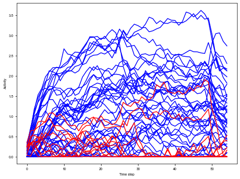
Plot neural activity from sample trials

trial = 2
plt.figure(figsize=(8, 6))
_ = plt.plot(activity_dict[trial][:, :net.e_size], color='blue', label='Excitatory')
_ = plt.plot(activity_dict[trial][:, net.e_size:], color='red', label='Inhibitory')
plt.xlabel('Time step')
plt.ylabel('Activity')
plt.show()

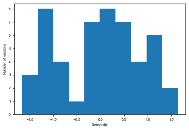
Compute stimulus selectivity for sorting neurons

Here for each neuron we compute its stimulus period selectivity \(d'\)

mean_activity = []
std_activity = []
for ground_truth in [0, 1]:
  activity = np.concatenate(stim_activity[ground_truth], axis=0)
  mean_activity.append(np.mean(activity, axis=0))
  std_activity.append(np.std(activity, axis=0))

# Compute d'
selectivity = (mean_activity[0] - mean_activity[1])
selectivity /= np.sqrt((std_activity[0] ** 2 + std_activity[1] ** 2 + 1e-7) / 2)

# Sort index for selectivity, separately for E and I
ind_sort = np.concatenate((np.argsort(selectivity[:net.e_size]),
                           np.argsort(selectivity[net.e_size:]) + net.e_size))

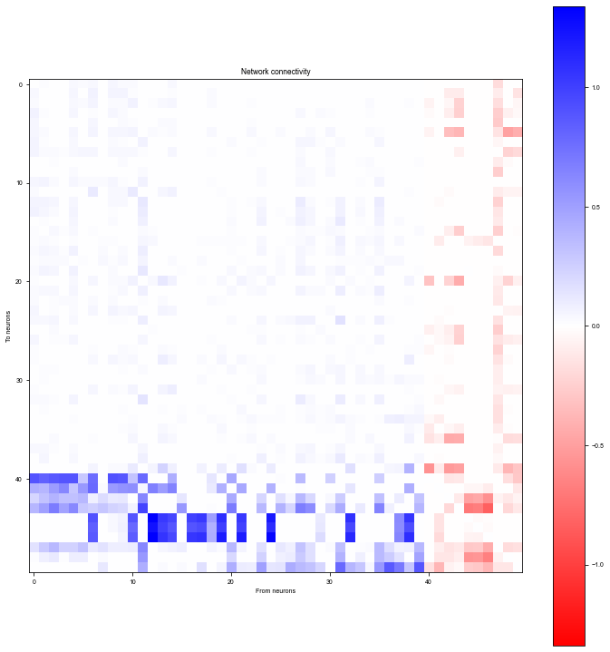
Plot network connectivity sorted by stimulus selectivity

# Plot distribution of stimulus selectivity
plt.figure(figsize=(6, 4))
plt.hist(selectivity)
plt.xlabel('Selectivity')
plt.ylabel('Number of neurons')
plt.show()

W = (bm.abs(net.w_rr) * net.mask).numpy()
# Sort by selectivity
W = W[:, ind_sort][ind_sort, :]
wlim = np.max(np.abs(W))

plt.figure(figsize=(10, 10))
plt.imshow(W, cmap='bwr_r', vmin=-wlim, vmax=wlim)
plt.colorbar()
plt.xlabel('From neurons')
plt.ylabel('To neurons')
plt.title('Network connectivity')
plt.tight_layout()
plt.show()